Effective Hamiltonian

In WimPyDD an Effective Hamiltonian can be initialized by instantiating the class eft_hamiltonian, which takes two arguments:

• a string with the Hamiltonian name
• a Python dictionary wc with the operators and the Wilson coefficients

 >>> hamiltonian=WD.eft_hamiltonian(string,wc)

Input

• wc={n1: func1 , n2: func2, ... }
n1,n2... identify the operators
func1, func2, ... are functions of the parameters \(w_i\), \(q\) that return the corresponding Wilson coefficients \(c^0,c^1\) in GeV\(^{-2}\)

The Hamiltonian can be written either in the base of Anand et al, or in that of Gondolo et al

Operator base of Anand et al,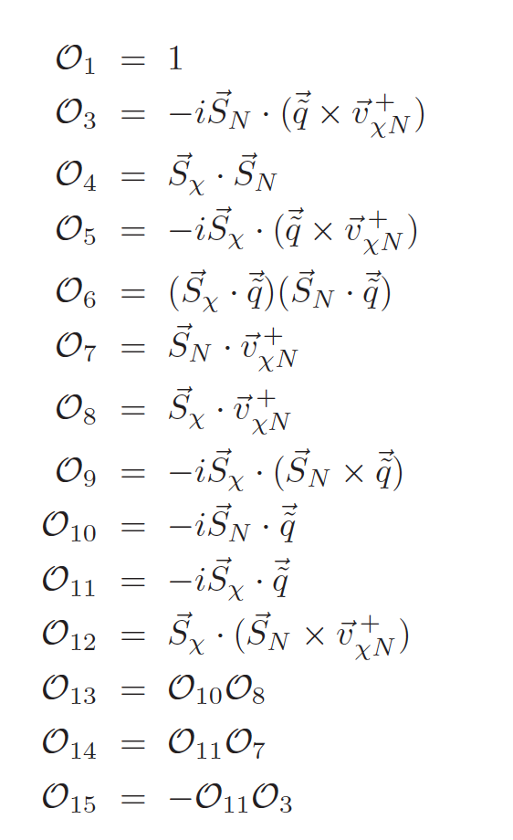

The keys n1, n2,...of the input dictionary must be integers picked by the list, [1,3,4,5,6,7,8,9,10,11,12,12,14,15]

Operator base of Gondolo et al,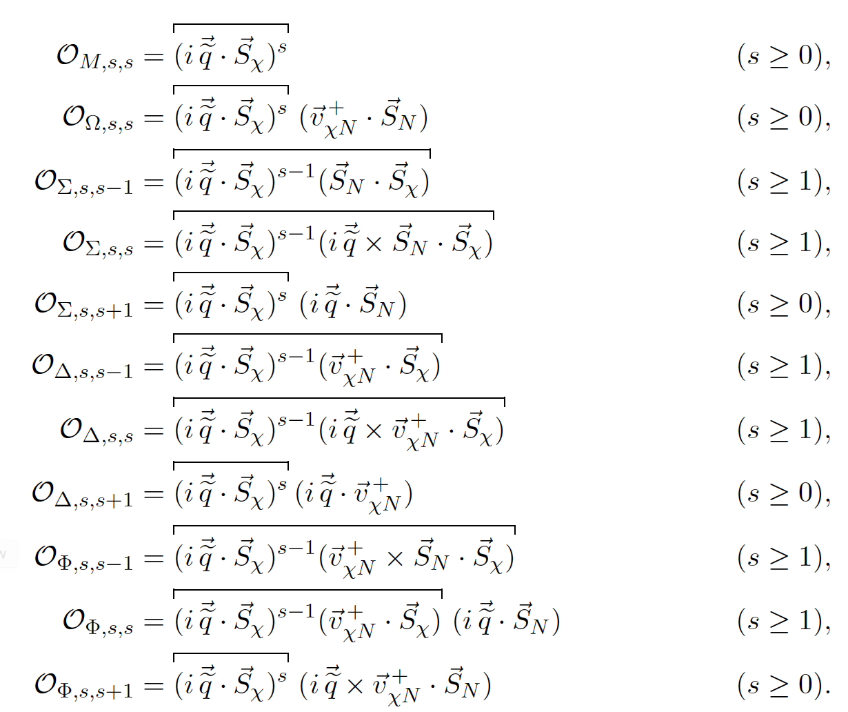

The keys n1,n2,...of the input dictionary must be tuples (X,s,l) with,

• X = string identifying the nuclear current with possible values X ='M','Omega','Sigma','Delta' and 'Phi'
• s = rank of the operator with possible values: s=0,1,...,2*j_chi with j_chi=\(j_\chi\) the spin of the WIMP
• l = power of the transferred momentum \(q\) in the operator with possible values:
  l = s for X = 'M', 'Omega'
  l=s-1, s, s+1 for X = 'Sigma', 'Phi'
  l=s-1, s for X = 'Delta'

Example: Anapole Dark Matter

1. In the base of arXiv:1308.6288 the effective Hamiltonian is given by:
\[ {\cal H} = \sum_{\tau=0,1} \left ( c_8^\tau {\cal O}_8^\tau+ c_9^\tau {\cal O}_9^{\tau}\right) \] \[c_8^\tau = \frac{2eg}{\Lambda^2} \, e^\tau, c_9^\tau = - \frac{eg}{\Lambda^2} \, g^\tau\] \[e^0=e^1=1,\] \[g^0=g_{\rm p}+g_{\rm n},~g^1=g_{\rm p}-g_{\rm n},\] where, \[g_{\rm p}=5.585\,694\,713(46), g_{\rm n}=-3.826\,085\,45(90),\] \[\alpha = e^2 / 4 \pi \simeq 1/137\] The interaction strength depends on \(g/\Lambda^2\) that can be parameterized in terms of the effective cross section \( \sigma_{\rm ref}\) and the WIMP mass \(m_\chi\): \[ \sigma_{\rm ref} \equiv \frac{2 \mu_{\chi N}^2 \, \alpha g^2 }{ \Lambda^4} \] with \(\mu_{\chi N}\) the WIMP-nucleon reduced mass.


Defining the two functions c8_anapole(mchi,sigma_ref) and c9_anapole(mchi,sigma_ref) (see here for an example of their implementation) the Hamiltonian is given by:



 >>> wc_anapole={8: c8_anapole, 9: c9_anapole}

 >>> anapole=WD.eft_hamiltonian('anapole',wc_anapole)

 >>> print(anapole)

     Hamiltonian name:anapole

     Hamiltonian:c8_anapole(mchi, sigma_ref)* O_8+c9_anapole(mchi, sigma_ref)* O_9

     Squared amplitude contributions:

     O_8*O_8, O_8*O_9, O_9*O_9



2. The same Hamiltonian can be expressed in the base of Gondolo et al,
\[{\cal H} = \sum_{\tau=0,1} \left ( c_{\Delta,1,0}^\tau {\cal O}_{\Delta,1,0}^\tau+ c_{\Sigma,1,1}^\tau {\cal O}_{\Sigma,1,1}^{\tau}\right)\]

so that:

 >>> wc_anapole_2={('Delta',1,0): c8_anapole, ('Sigma',1,1): c9_anapole}

 >>> anapole_2=WD.eft_hamiltonian('anapole_2',wc_anapole_2)

 >>> print(anapole_2)

     Hamiltonian name:anapole_2

     Hamiltonian:c8_anapole(mchi, sigma_ref)* O_Delta_1_0
                 +c9_anapole(mchi, sigma_ref)* O_Sigma_1_1

     Squared amplitude contributions:

     O_Delta_1_0*O_Delta_1_0, O_Delta_1_0*O_Sigma_1_1, O_Sigma_1_1*O_Sigma_1_1

leads to the same result.

 >>> WD.load_response_functions(WD.XENON_1T_2018, anapole, j_chi=0.5)

loads or saves the following files in the directory

 >>> WD.load_response_functions(WD.XENON_1T_2018,anapole_2,j_chi=0.5)

loads and/or saves:

in the same directory.

 >>> H8=WD.eft_hamiltonian('H8',{8: lambda M,g,r=1: g/M**2*np.array([1+r,1-r])})  

Main attributes and methods of the eft_hamiltonian class

For the anapole and anapole_2 hamiltonians defined above:

 >>> [attr for attr in dir(anapole) if '__' not in attr]

     ['arguments', 'coeff_squared', 'coeff_squared_list', 'coeff_squared_q_dependence', 

      'couplings', 'default_args', 'global_arguments', 'global_default_args', 

      'hamiltonian', 'name', 'print_hamiltonian', 'print_hamiltonian_latex', 

      'wilson_coefficients']

 >>> anapole.coeff_squared(8,9,mchi=100,sigma_ref=1e-40) 

     array([[-6.68076649e-12, -3.57340160e-11],

     [-6.68076649e-12, -3.57340160e-11]])

 >>> anapole_2.coeff_squared((('Delta',1,0)),('Sigma',1,1),mchi=100,sigma_ref=1e-40) 

 >>> anapole.coeff_squared_list

     [(8, 8), (8, 9), (9, 9)]

 >>> anapole_2.coeff_squared_list

     [(('Delta', 1, 0), ('Delta', 1, 0)), (('Delta', 1, 0), ('Sigma', 1, 1)),

     (('Sigma', 1, 1), ('Sigma', 1, 1))] 

Returns a list of the contributions \({\cal O}_j{\cal O}_k\) to the squared amplitude.

 >>> anapole.coeff_squared_q_dependence(0.1,8,9) 

Calculates the factorized momentum dependence of the product \(c_8^{\tau}c_9^{\tau^{\prime}}\).

 >>> anapole_2.coeff_squared_q_dependence(0.1,('Delta',1,0),('Sigma',1,1)) 

Calculates the same quantity for \(c_{\Delta,1,0}^{\tau}c_{\Sigma,1,1}^{\tau^{\prime}}\). Return 1 if the Wilson coefficients do not depend on \(q\).

 >>> wc={5 : lambda cp=1, cn=1, M=10**3: 1/M**2*np.array([cp+cn,cp-cn])}

Once the Wilson is defined user can write the EFT hamiltonian as:

 >>> c5=WD.eft_hamiltonian('c5', wc) 

Here \(c_p\) and \(c_n\) are the WIMP couplings to proton and neutron respectively while \(M\) is any effective scale. As usual a short summary of effective_hamiltonian can be obtained by printing it:

 >>> print(c5)

     Hamiltonian name:c5

     Hamiltonian:c_5(cp=1, cn=1, M=1000)* O_5

     Squared amplitude contributions:

     O_5*O_5

In the case of more than one interactions the user can define the Wilson coefficients as following:

 >>> wc={8 : lambda cp=1, cn=1, q=1: 1/q**2*np.array([cp+cn,cp-cn]),

     9 : lambda cp=1, cn=1: np.array([cp+cn,cp-cn])})

which leads to the following hamiltonian:

 >>> c8_c9=WD.eft_hamiltonian('c8_c9', wc) 

As metioned before a short summary of EFT hamitonian can be obtained using print option:

 >>> print(c8_c9)

     Hamiltonian name:c8_c9

     Hamiltonian:c_8(cp=1, cn=1, q=1)* O_8'(q)+c_9(cp=1, cn=1)* O_9

     Squared amplitude contributions:

     O_8'(q)*O_8'(q), O_8'(q)*O_9, O_9*O_9

Notice that the operator \(\mathcal{O}_8\) depends on the transfer momentum (here a long range interaction) while \(\mathcal{O}_9\) is independent of that. A cautious user might have already noticed an interference term between \(\mathcal{O}_8\) and \(\mathcal{O}_9\) operators that is expected following EFT approach.

The arguments of the defined Hamiltonian can be accessed by following:

 >>> c8_c9.arguments 

     {8: ['cp', 'cn', 'q'], 9: ['cp', 'cn']}

If the value of an argument is not defined by the user it will be put to 1 by default. Notice that user should not pass the value of momentum transfer \(q\) in the argument as \(q\) is used in the calcualtion of the response functions and treated differently inside WimPyDD. But user has freedom to change any other arguments for example \(c_p, c_n\) here.

Once the Nuclear Target and Effective Hamiltonian are defined, the user could move on to define an Experiment.